This short snapshot simply provides a reference of using the FILTER function in Excel.
Keep in mind, this reference does not go into full detail of using this function. On the whole, it is a snapshot of the function. We pattern this example from the following function.
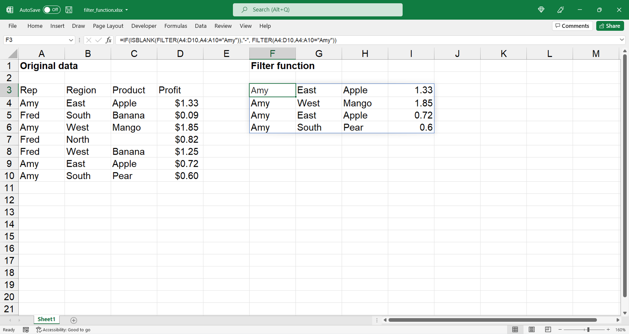
Snapshot of using the FILTER function
Below is a small snapshot of the FILTER function. It allows you to separate a range of data based on criteria you define. Also, it is a function introduced to Excel for Microsoft 365.
The list
Here is the list from the above image. So, feel free to copy it into Excel, to practice.
| Rep | Region | Product | Profit |
|---|---|---|---|
| Amy | East | Apple | $1.33 |
| Fred | South | Banana | $0.09 |
| Amy | West | Mango | $1.85 |
| Fred | North | $0.82 | |
| Fred | West | Banana | $1.25 |
| Amy | East | Apple | $0.72 |
| Amy | South | Pear | $0.60 |
The function
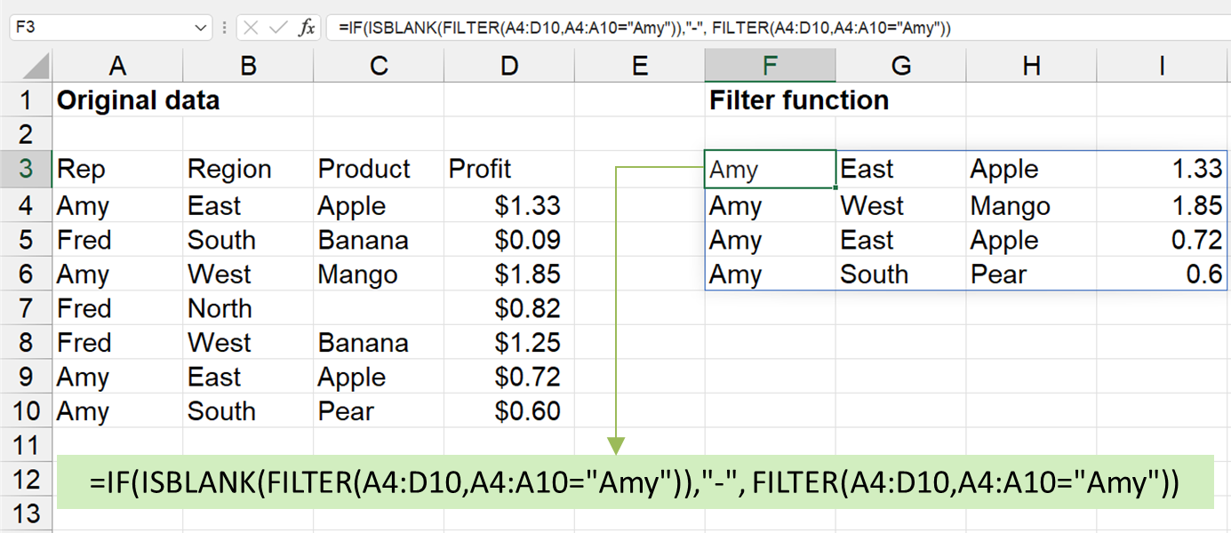
Below is the function to show data based on certain criteria, in this example. Also, copy it to Excel to practice.
=IF(ISBLANK(FILTER(A4:D10,A4:A10=”Amy”)),”-“, FILTER(A4:D10,A4:A10=”Amy”))
As you see, the results of this function shows another list. Since it lists a set of data, you can look at this function as a dynamic array. And, the list generally starts wherever you enter the formula.